
Using Linear Weights to Evaluate Hitters
Not all hits (or hitters) are created equal


Quick note: It’s been brought to my attention that some of these posts are too long for email. Because of this, I highly encourage you to download the substack app and read these there (click “get the app” below) - or on my actual substack page on the website (link).
By mere reason, I conceded long ago that there are more comprehensive ways to use statistics that better capture a player's offensive value1 (compared to traditional counting statistics). One such method is using a model with linear weights, which allows us to assign more precise values to each of a hitter's individual actions. And as the title already suggested, this will be the focus of today’s post.
What Are Linear Weights?
A linear weight is a statistical method that uses a weighted sum of offensive events - like singles, doubles, triples, home runs, walks, and more - to estimate how many runs a player generates for their team. In essence, it’s a system designed to quantify the value of each outcome during a hitter’s plate appearance and asses how much each event contributes to scoring runs.
The term linear weights comes from the statistical technique of linear regression, which aims to find the best linear relationship between a set of independent variables (such as, in this case, hits, walks, etc.) and a dependent variable (in this case, generated runs).
Analysts apply this concept to baseball by analyzing historical data to determine each offensive event's average impact on run production.
The Foundation of Linear Weights
To understand how linear weights work, let’s break down the approach step by step:
Step 1: Regression Model:
Team analysts use regression models to predict the number of runs a team or a player will score/generate based on various offensive events. The model looks something like this:
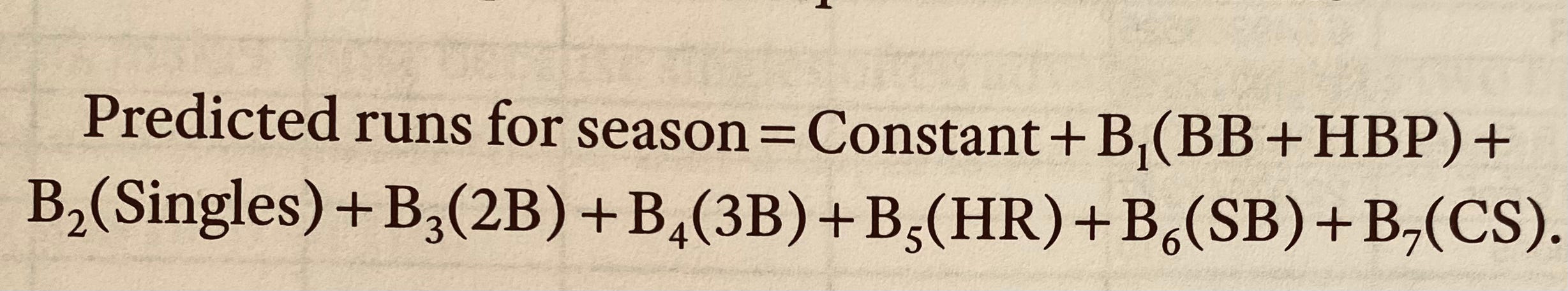
As we stated earlier, the variables (BB, 1B, etc.) are the independent variables, and the goal is to predict the dependent variable, which is team/player runs scored/generated. The weights (B1, B2, etc.) are the coefficients assigned to each event, representing how much that event is worth in terms of run production.
Step 2: Determining the Value of Each Event:
Below are assigned values for each event with a brief explanation. I’m using MLB historical data from 2000 to 2006 for this example.2
Single = 0.63 runs
A Single allows the batter to reach first base, often advancing other runners on base and sometimes contributing directly to scoring runs. While it doesn’t guarantee runners will score, it creates opportunities by keeping the inning alive and potentially moving runners into scoring position, which makes it more valuable than a walk or a non-hit event but less than any XBHs.
Double = 0.72 runs
A Double, on average, advances base runners more effectively than a single but does not have the guaranteed run-scoring potential of a home run. Doubles typically allow runners on base to advance two bases, often putting them in scoring position or driving them in, which is why its value is higher than a single (0.63 runs).
Triple = 1.24 Runs
A Triple almost guarantees that a batter will score after reaching third base while also frequently driving in other runners on base. The value reflects that a triple not only puts the batter in prime scoring position but also has a high likelihood of directly generating runs, though it’s slightly less valuable than a home run, which results in an immediate score.
Home Run = 1.50 Runs
A Home Run guarantees the batter scores and brings in any runner already on base. The value is based on the fact that a home run always results in at least one run (the batter), and with an average of one runner on base, it often leads to additional runs being scored.
Walks + HBP = 0.35 Runs
Walks + HBP allow the batter to reach base without making an out, which helps extend the innings and creates opportunities for other runners to advance. While walks + HBP don’t directly move runners as far as hits do, they still contribute run production by putting additional players on base and sometimes advancing runners already on base.
Stolen Base = 0.06 Runs
A Stolen Base, while it does advance a runner into a better scoring position, has a relatively small overall impact on run production compared to hits or other offensive events. Stolen Bases slightly increase the chance of scoring, but they don’t directly generate runs and come with the risk of being caught stealing.
Caught Stealing = -0.02
While Caught Stealing results in an out and eliminates a base runner, the overall negative impact on run production is relatively small when averaged over many games. This small value reflects that, although being caught stealing disrupts the inning and reduces scoring opportunities, it typically doesn’t have as severe an impact as other negative events like strikeouts or double plays.
Step 3: The Equation
After performing a regression analysis on the data, we can then complete our equation…
Predicted Runs = −563.03 + 0.63 (singles) + 0.72 (doubles) + 1.24 (triples) + 1.50 (home runs) + 0.35 (walks + hit by pitch) + 0.06 (stolen bases) + 0.02 (caught stealing)
Using this equation3, we can now better evaluate both a player’s and a team’s offensive output.
Example: Derek Jeter vs Albert Pujols
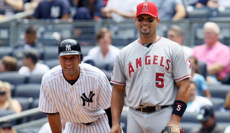
Ok, now for some fun. Let’s evaluate and compare the careers of one hall of famer, Derek Jeter, and Albert Pujols, who should be a first-ballot Hall of Famer in 2028. Both players had long, illustrious careers, but they were very different types of hitters. By using linear weights, we can attempt to better quantify the value each player added to their teams’ run production over the course of their careers.
Below are the lifetime totals for the relevant offensive categories for our model:
Now, using our weights above, let’s calculate the runs created for each player by multiplying their career totals by the linear weights coefficients:
Derek Jeter
Singles: 2,595 × 0.63 = 1,634.85 runs
Doubles: 544 × 0.72 = 391.68 runs
Triples: 66 × 1.24 = 81.84 runs
Home Runs: 260 × 1.50 = 390 runs
Walks + HBP: 1,082 × 0.35 = 378.7 runs
Stolen Bases: 358 × 0.06 = 21.48 runs
Caught Stealing: 97 × (-0.02) = -1.94 runs
Total Runs Created = 1,634.85 + 391.68 + 81.84 + 390 + 378.7 + 21.48 - 1.94
= 2,896.61 runs
Albert Pujols:

Singles: 2,073 × 0.63 = 1,306.35 runs
Doubles: 686 × 0.72 = 493.92 runs
Triples: 16 × 1.24 = 19.84 runs
Home Runs: 703 × 1.50 = 1,054.5 runs
Walks + HBP: 1,373 × 0.35 = 480.55 runs
Stolen Bases: 117 × 0.06 = 7.02 runs
Caught Stealing: 55 × (-0.02) = -1.1 runs
Total Runs Created= 1,306.35 + 493.92 + 19.84 + 1,054.5 + 480.55 + 7.02 - 1.1
= 3,361.08 runs
Analysis
Total Offensive Value:
With 3,361.08 total runs created, Pujols contributed 464.47 more runs to his team than Derek Jeter, who created 2,896.61 runs. Pujols’ superior power numbers (703 career home runs) and XBHs were clearly the difference. From a scouting perspective, this is an excellent example of why the Impact (Power) grade is so important when scouting for the amateur draft. By the 20-80 scouting scale standards, Albert Pujols is what an 80-grade (elite) power hitter looks like, whereas Jeter was more of a 40-grade (slightly below average) power guy. Slugging the baseball is incredibly valuable.
Power vs Contact:
Jeter was known for his contact ability, as seen in his 2,595 career singles (out of 3,465 career hits). However, compared to Pujols' 2,072 singles (out of 3,384 career hits), it's not exactly superior to Pujols. Pujols' 703 home runs (weighted at 1.50 runs each) give him a significant edge in terms of offensive impact. Pujols also hit 686 doubles compared to Jeter's 544, further widening the gap in extra-base hit production.
Walks and Discipline:
Pujols also has a notable advantage in walks and hit-by-pitch numbers (1,373 to Jeter’s 1,082), contributing additional value to his ability to get on base.
Speed and Base Running:
Jeter holds the advantage in stolen bases (358 to 117), and although the impact of stolen bases is relatively small in the model, it does show that Jeter added a good amount of value with his legs.
Interpretation:
Although this is not the entire picture, using linear weights can be a much better way to evaluate hitters than merely the traditional "counting" statistics. For example, Jeter slashed a very nice .310/.377/.440 in his career, while Pujols slashed .296/.374/.544. From the traditional lens, Derek Jeter looks like the better player, with the argument championing his higher batting average. However, using our model, we know that in Pujols' 22-year career, he created 464.47 more runs for his team than Jeter did in his 20-year career.
My interpretation of this case study is this: 1) Albert Pujols should be a first-ballot Hall-of-Famer, and 2) the most productive players in Major League Baseball are typically ones who can slug. Home runs and extra-base hits will win your team ball games. However, I'm not saying that contact-first-focused hitters aren't valuable. They most certainly are. However, the biggest risk with being a contact-first hitter in Major League Baseball is that in order to really contribute to your club's offense, you have to be really, really... really good at it.
As we’ll see in the next example.
An Emphasis
To emphasize the point in my interpretation, let’s take a look at two very different types of leadoff hitters’ 2024 season: Kyle Schwarber, who slashed .248/.366/.485 this season, and Luis Arraez, who slashed .314/.346/.392 - and who was also the 2024 NL Batting Champ (award given to the player with the highest batting average).
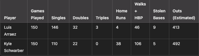
Now, using the same linear weight values as before, let’s estimate the runs created by each player…
Luis Arraez:

Singles: 146 × 0.63 = 91.98 runs
Doubles: 32 × 0.72 = 23.04 runs
Triples: 3 × 1.24 = 3.72 runs
Home Runs: 4 × 1.50 = 6 runs
Walks + HBP: 46 × 0.35 = 16.10 runs
Stolen Bases: 9 × 0.06 = 0.54 runs
Total Runs Created = 91.98 + 23.04 + 3.72 + 6 + 16.10 + 0.54
= 141.38 runs
Kyle Schwarber:

Singles: 110 × 0.63 = 69.30 runs
Doubles: 22 × 0.72 = 15.84 runs
Triples: 0 × 1.24 = 0 runs
Home Runs: 38 × 1.50 = 57 runs
Walks + HBP: 106 × 0.35 = 37.10 runs
Stolen Bases: 5 × 0.06 = 0.30 runs
Total Runs Created = 69.30 + 15.84 + 0 + 57 + 37.10 + 0.30
= 179.54 runs
Now, knowing this information, I ask…
Who would you rather have on your team and as your leadoff hitter?
The 2022, 2023, and 2024 Batting Champ?
Or, the .248 hitter (who also has never hit above .300 in his life)?
If your goal is to have the highest team batting average in baseball - you would pick Luis Arraez.
HOWEVER, if your goal is to score more runs and to win more baseball games (to win a World Series!) - based on this information, you would want to pick the career .230 hitter…

Points of Fragility
Having said all of this, we must remember that the best analyst are not the ones with the most sophisticated models, the best analyst are the ones who understand where the models are most fragile. Therefore, to end this post, let’s examine some points of fragility when using linear weight models:
Context-Independent Valuation of Events4
Linear Weight models assume that the run value of an event (e.g., a home run, single, or walk) is independent of the game context. For instance, a home run is always valued at 1.50 runs, regardless of when it occurs or the situation on the field. This approach provides a simplified, average-based understanding of how offensive events contribute to scoring over many games and seasons.
Point of Fragility:
In real-world situations, the value of a particular event can vary greatly depending on the game context. A home run in the bottom of the ninth inning of a tied game could effectively win the game, (theoretically) making it far more valuable than a home run in the first inning of a blowout. In high-leverage situations, the impact of an event extends beyond its raw contribution to runs; it can influence game outcomes and even playoff standings.
Reliance on Historical Data
Linear Weights are based on past data, which can introduce a potential point of fragility when forecasting future outcomes.
Point of Fragility:
Player performance can fluctuate due to various factors, including rule changes, making the results of a given season potentially misleading when projecting future performance. Recent examples of significant rule changes in baseball highlight how historical data may not always be a reliable predictor of future outcomes.
In the next post, we’ll talk about evaluating hitters using a Monte Carlo Simulation.
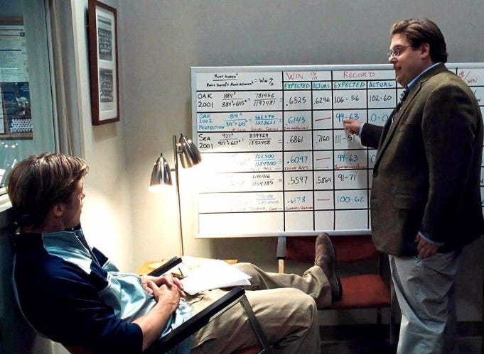
Until then, remember, as the fictionalized (and sensationalized) character of Billy Beane (played by an incredibly over-rated actor) said in the movie Moneyball, no matter what your evaluation process is…

Happy Playoffs.
Which through this process, I also discovered how mediocre of a player I was.
There’s no specific reason why I’m using this dataset other than I have it in front of me at the moment.
The constant in a regression equation, such he -56.03 in this runs predicted formula, is known as the “intercept.” In the context of this regression, it represents the baseline value when all of the independent variables (walks, singles, doubles, home runs, etc.) are zero. In short, the constant (-563.03) is just a mathematical adjustment that aligns the regression model with the actual data, ensuring the formula accurately predicts runs based on offensive events.
Some may scoff at this, but I think it deserves highlighting.